Amazon Timestream vs DynamoDB for Timeseries Data

Update 30. November 2021: AWS has released multi-measure records, scheduled queries, and magnetic storage writes for Amazon Timestream.

AWS recently announced that their Timestream database is now generally available. I tried it out with an existing application that uses timeseries data. Based on my experimentation this article compares Amazon Timestream with DynamoDB and shows what I learned.

Timeseries data is a sequence of data points stored in time order. Each timestream record can be extended with dimensions that give more context on the measurement. One example are fuel measurements of trucks, with truck types and number plates as dimensions.

Prerequisites

As this article compares Timestream with DynamoDB, it’s good for you to have some experience with the latter. But even if you don’t, you can learn about both databases here.

I will also mention Lambda and API Gateway. If you’re not familiar with those two, just read them as “compute” and “api”.

Use Case

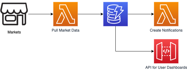
My application monitors markets to notify customers of trading opportunities and registers about 500,000 market changes each day. DynamoDB requires ~20 RCU/WCUs for this. While most of the system is event-driven and can complete eventually, there are also userfacing dashboards that need fast responses.

Below you can see a picture of the current architecture, where a Lambda function pulls data into DynamoDB, another one creates notifications when a trading opportunity appears and an API Gateway that serves data for the user dashboards.

Each record in the database consists of two measurements (price and volume), has two dimensions (article number and location) and has a timestamp.

Testing out Timestream required two changes: An additional Lambda function to replicate from DynamoDB to Timestream, and a new API that reads from Timestream.

Data Format

Let’s start by comparing the data format of DynamoDB and Timestream.

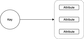
DynamoDB holds a flexible amount of attributes, which are identified by a unique key. This means that you need to query for a key, and will get the according record with multiple attributes. That’s for example useful when you store meta information for movies or songs.

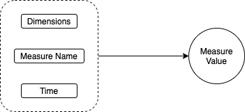
Timestream instead is designed to store continuous measurements, for example from a temperature sensor. There are only inserts, no updates. Each measurement has a name, value, timestamp and dimensions. A dimension can be for example the city where the temperature sensor is, so that we can group results by city.

Write to Timestream

Timestream shines when it comes to ingestion. The WriteRecords API is designed with a focus on batch inserts, which allows you to insert up to 100 records per request. With DynamoDB my batch inserts were sometimes throttled both with provisioned and ondemand capacity, while I saw no throttling with Timestream.

Below you can see a snapshot from AWS Cost Explorer when I started ingesting data with a memory store retention of 7 days. Memory store is Timestream’s fastest, but most expensive storage. It is required for ingestion but its retention can be reduced to one hour.

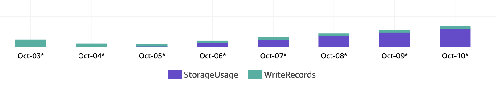
The write operations are cheap and can be neglected in comparison to cost for storage and reading. Inserting 515,000 records has cost me $0.20, while the in-memory storage cost for all of those records totalled $0.37 after 7 days. My spending matches Timestream’s official pricing of $0.50 per 1 million writes of 1KB size.

As each Timestream record can only contain one measurement, we need to split up the DynamoDB records which hold multiple measurements. Instead of writing one record with multiple attributes, we need to write one record per measure value.

Backfilling old data might not be possible if its age exceeds the maximum retention time of the memory store which is 12 months. In October 2020 it was only possible to write to memory store and if you tried to insert older records you would get an error. To backfill and optimize cost you can start with 12 months retention and then lower it once your backfilling is complete.

Read from Timestream

You can read data from Timestream with SQL queries and get charged per GB of scanned data. WHERE clauses are key to limiting the amount of data that you scan because “data is pruned by Amazon Timestream’s query engine when evaluating query predicates” (Timestream Pricing).

The less data makes it through your WHERE clauses, the cheaper and faster your query.

I tested the read speed by running the same queries against two APIs that were backed by DynamoDB (blue) and Timestream (orange) respectively. Below you can see a chart where I mimicked user behavior over the span of an hour. The spikes where DynamoDB got slower than Timestream were requests where computing the result required more than 500 queries to DynamoDB.

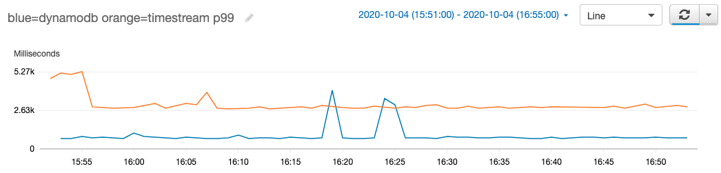
DynamoDB is designed for blazing fast queries, but doesn’t support adhoc analytics. SQL queries won’t compete at getting individual records, but can get interesting once you have to access many different records and can’t precompute data. My queries to Timestream usually took more than a second, and I decided to precompute user facing data into DynamoDB.

Dashboards that update every minute or so and can wait 10s for a query to complete are fine with reading from Timestream. Use the right tool for the right job.

Timestream seems to have no limit on query length. An SQL query with 1,000 items in an SQL IN clause works fine, while DynamoDB limits queries to 100 operands.

Timestream Pricing

Timestream pricing mostly comes down to two questions:

• Do you need memory store with long retention?
• Do you read frequently?

Below you can see the cost per storage type calculated into hourly, daily and monthly cost. On the right hand side you can see the relative cost compared to memory store.

My ingestion experiments with Timestream were quite cheap with 514,000 records inserted daily for a whole month and the cost ending up below $10. This is a low barrier to entry for you to make some experiments. I dropped the memory storage down to two hours, because I only needed it for ingestion. Magnetic store seemed fast enough for my queries.

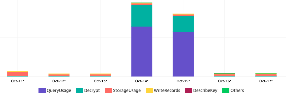
When I tried to read and precompute data into DynamoDB every few seconds, I noticed that frequent reads can become expensive. Timestream requires you to pick an encryption key from the Key Management Service (KMS), which is then used to decrypt data when reading from Timestream. In my experiment decrypting with KMS accounted for about 30% of the actual cost.

Below you can see a chart of my spending on Timestream and KMS with frequent reads on October 14th and 15th.

Problems and Limitations

Records can get rejected for three reasons:

• Duplicate values for the same dimensions, timestamps, and measure names
• Timestamps outside the memory’s retention store
• Dimensions or measures that exceed the Timestream limits (e.g. numbers that are bigger than a BigInt)

Based on my experience with these errors I suggest that you log the errors but don’t let the exception bubble up. If you’re building historical charts, one or two missing values shouldn’t be a problem.

Below you can see an example of how I write records to Timestream with the boto3 library for Python.

import boto3

timestream = boto3.client('timestream-write')

try:
    timestream.write_records(
        DatabaseName='MarketWatch',
        TableName='Snapshots',
        CommonAttributes={
            'Time': str(int(time())),
            'TimeUnit': 'SECONDS'
        },
        # each chunk can hold up to 100 records
        Records=chunk
    )
except client.exceptions.RejectedRecordsException as err:
    print({'exception': err})
    for rejected in err.response['RejectedRecords']:
        print({
            'reason': rejected['Reason'],
            'rejected_record': chunk[rejected['RecordIndex']]
        })

Another perceived limitation is that each record can only hold one measurement (name and value). Assuming you have a vehicle with 200 sensors, you could write that into DynamoDB with one request, while Timestream already needs two. However this is pretty easy to compensate and I couldn’t come up with a good acceess pattern where you must combine different measurement types (e.g. temperature and voltage) in a single query.

Last but not least, Timestream does not have provisioned throughput yet. Especially when collecting data from a fleet of IoT sensors it would be nice to limit the ingestion to not cause cost spikes that may be caused by a bug in the sensors. In my tests the cost for writing records has been negligible though.

Summary

I moved my timeseries data to Timestream, but added another DynamoDB table for precomputing user facing data. While my cost stayed roughly the same, I now have cheap long term storage at 12% of the previous price.

DynamoDB is faster for targeted queries, whereas Timestream is better for analytics that include large amounts of data. You can combine both and precompute data that needs fast access.

Trying out queries is key to understanding if it fits your use case and its requirements. You can do that in the timestream console with the AWS examples. Beware of frequent reads and monitor your spending.

Try it out

Try out one of the sample databases through the Timestream console or replicate some of the data you write to DynamoDB into Timestream. You can achieve the latter for example with DynamoDB streams.

For some more inspiration, check out the timestream tools and samples by awslabs on GitHub.

Further Reading

• Timestream now Generally Available
• Unboxing Amazon Timestream
• Design patterns for high-volume, time-series data in Amazon DynamoDB
• Best Practices for Implementing a Hybrid Database System

Enjoyed this article? I publish a new article every month. Connect with me on Twitter and sign up for new articles to your inbox!